- You are here:
- Home »
- Blog »
- Power BI »
- Connecting to Web Page Data in Power BI
Connecting to Web Page Data in Power BI
As well as retrieving data from a web URL, Power BI also allows you to retrieve data from within the web page itself. In this tutorial article, we will see how easy it is to connect to online data and incorporate it into your own data models.
The files used in this tutorial can be downloaded from this URL:
https://drive.google.com/file/d/0BztAs7QVJD5tOTEwbnkyLW0xU3M/view?usp=sharing
Examining the Source Data
If you look in the tutorial folder you will find the Excel file called “Travel budget” which contains the data that we will be using in this example.
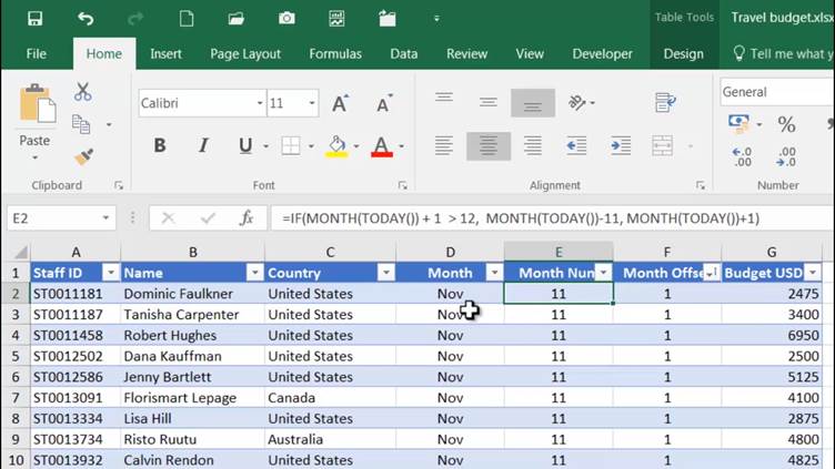
So here we have a table containing budget data which shows the estimated travel costs all our employees. To keep the data fresh, instead of putting static data in the “Month Num” column, I’ve actually just used a formula; so that, whenever you open the file, Excel recalculates the next three months. The figures in the “Budget USD” will stay the same, but the month columns will change depending on the current date.
So that’s the data with which we will be starting; and what we want to do is to extend this data so that, as well as having figures in US dollars, we can also have them in the currency of all the other countries in which our fictitious company is based: Australia, Canada, New Zealand and the United Kingdom.
Connecting to the Excel Data
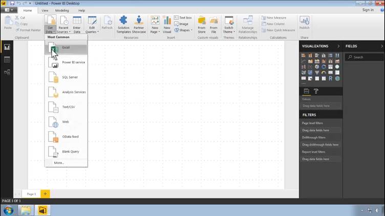
In Power BI, we choose Home > Get Data > Excel and navigate to the “Travel budget” file, then double-click to connect to it.
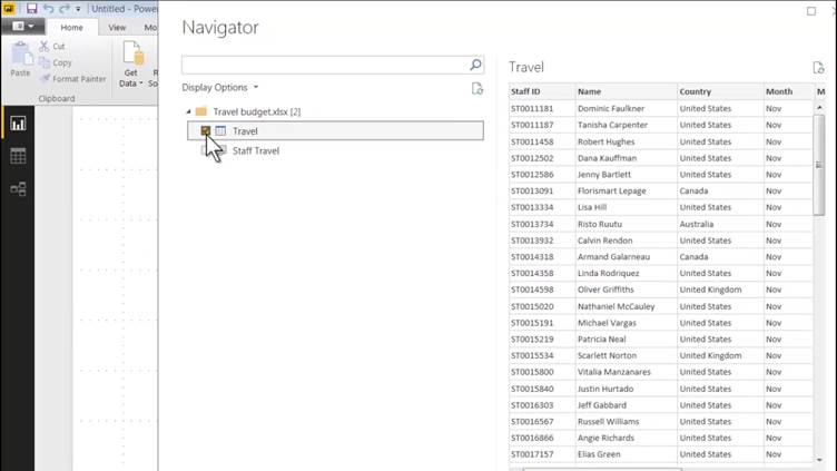
When Power BI displays the Navigator, we activate the checkbox next to the “Travel” table and click the Edit button to view the table in the Query Editor.
Connecting to the Currency Exchange Rate Data
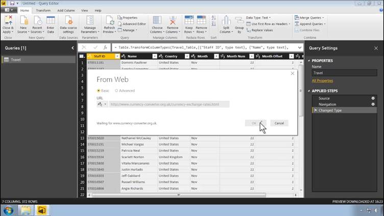
In the Query Editor, choose Home > New Source > Web. Enter the following URL and click OK to connect:
http://www.currency-converter.org.uk/currency-exchange-rates.html
Naturally, when examining the webpage, Power BI will focus on tabular data; basically, it is going to look for HTML tables; and it shows you all of the tables it has retrieved. When you click on the checkbox next to each one, you are given a preview of the data which that table contains.
The table we are looking for is the one which contains the exchange rate information. Power BI provides the useful facility, when you are connecting to webpages, of switching to web view, in which you are given a preview of the table as it appears on the webpage. This makes it fairly easy to locate the correct table; in our case, we need the table called “Foreign Currency Exchange Rates Today…”.
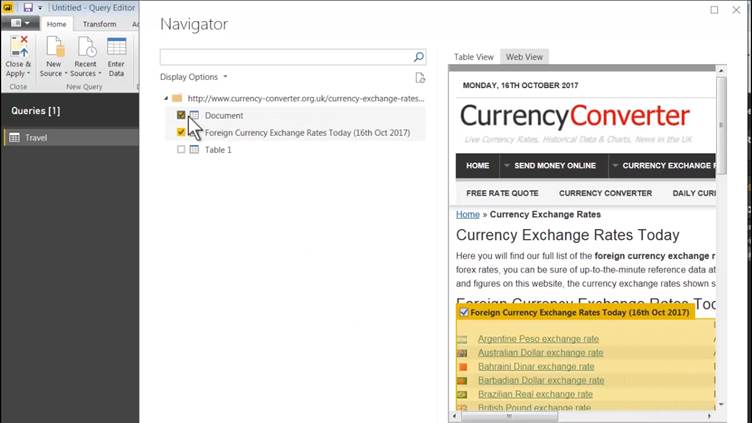
The table which we retrieve contains conversion rates for converting a number of different currencies into six major currencies: GBP, EUR, USD, AUD, NZD and CAD.
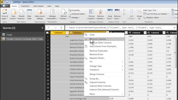
Query Editor: Remove Columns
Since we will not need the first two columns, we can simply highlight them, using click and then Control-click; then Right-click on a selected column header and choose Remove Columns from the context menu.
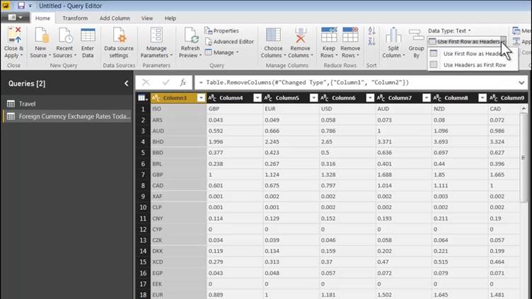
Query Editor: Use First Row as Headers
Next, we need to tell Power BI that the first row contains the column headings; and we do this by choosing Home > Use First Row as Headers.
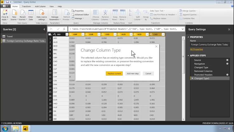
Query Editor: Change Type
Next we need to make sure that we have numeric values in the conversion rate columns; at the moment everything is still text. So, we select all of the numeric columns by clicking on the first and then Shift-clicking on the last. Then we Right-click and choose Change Type > Decimal Number and then just click on Replace Current to update the existing Change Type step.
We can also remove the EUR(Euro) column; because none of the countries in which our fictitious company operates are in the Eurozone.
Query Editor: Filtering out Unwanted Rows
Using the filter arrow on the right of the ISO column heading, we can now filter out all of the currencies which are not required. First, we use the Select All toggle, so that nothing is selected; then we activate only USD.
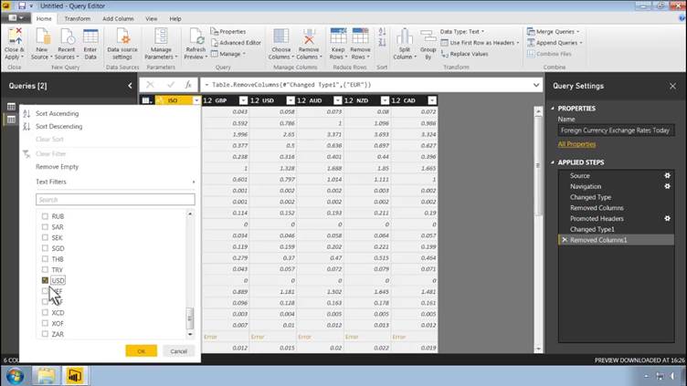
When we click OK, only one row is shown in the table; the one which contains the currency rates for converting dollars. (Since the dollar is our base currency, the only conversion we will actually be doing will be from US dollars into each of the other currencies.)

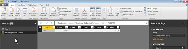
Query Editor: Renaming a Query
Queries are automatically assigned a name based on the underlying data source; so it is usually a good idea to rename them. To do this, we simply double-click on the current name (or select the query and press F2 on the keyboard) and enter a new one. Let us call the query “Exchange Rates Today”.
Query Editor: Creating a Custom Column
The final transformation which we will put in place is a mechanism for connecting the two tables. In order to connect the two tables, we will need to have a column in the “Travel” table which is equivalent to the ISO column in the “Exchange Rates Today” table.
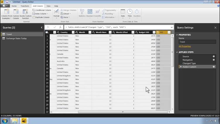
We do this by clicking on Add Column > General > Custom Column; and let’s call the new column “ISO”, to match the column in the other table. Now we simply need to make sure that the new column has the word “USD” in every row; and we do this by creating a formula which simply consists of that one literal value, which of course, being a string, has to be placed in double quotes.
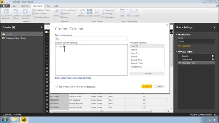
When we click OK, we have a new column at the on the right of the table called “ISO” containing “USD” in every row.
Thus, when we use this column to connect the two tables, every single row in the “Travel” table will match the single USD row in the “Exchange Rates Today” table; and then we can simply use the appropriate conversion to calculate a value in each of the required currencies.
Query Editor: Close and Apply
That is all we need to do in the Query Editor; so, to exit and save our changes, we click on File > Close & Apply.
Adding a Report Background
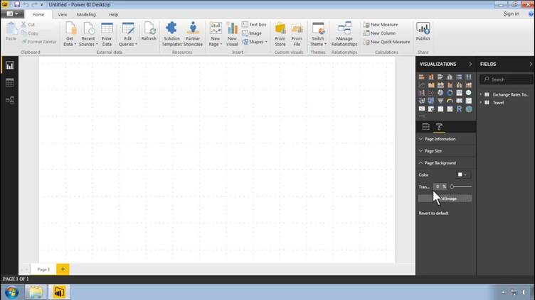
Now let us begin the creation of our report by inserting a background. In the Visualizations pane, expand the “Page Background” section by clicking on the arrow on the left of its label; and then click on the “+ Add Image” button.
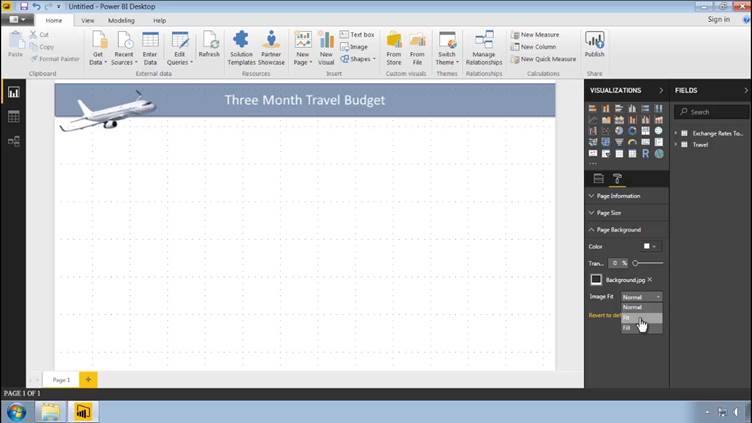
Next, navigate to the tutorial folder and double-click on the file called “Background.jpg”. You will find that the image is a close, but not exact, match for the page. To rectify this slight discrepancy, click Image Fit > Fit.
Automatic Detection of Relationships
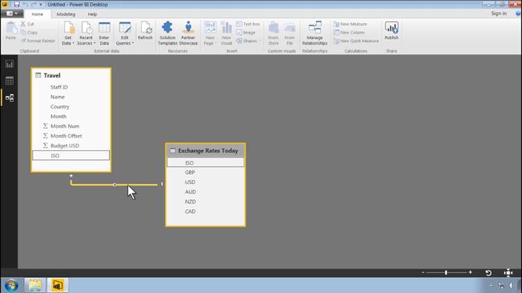
Next, we need to verify that the two tables are connected; and we do this by clicking on the Relationships icon on the left of the screen. The fact that we used the same name when creating the extra column in the travel table means that Power BI has automatically created the relationship for us; so the two tables are already linked using the common column that we engineered in the Query Editor.
Using the Table Visual
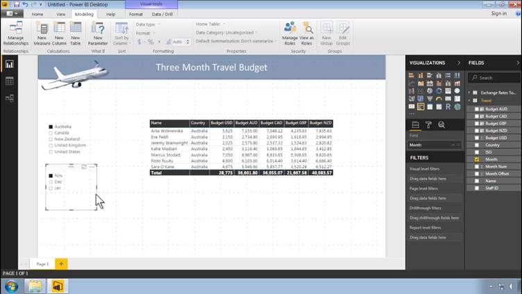
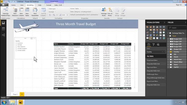
Now let us put together our basic report starting with a table. Click on the Table icon in the Visualizations pane. (The name of each visual is displayed as a tool tip as you hover over the icons.) Then increase the size of the tile and move it to the right of the page, as shown below.
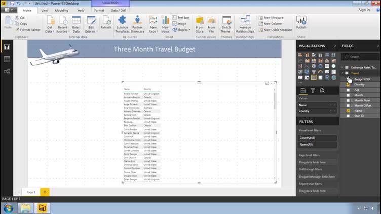
To populate the table, drag fields from the Fields pane into the “Values” section of the Visualizations pane. Let’s start with the name of each of the individuals (“Name”); their country (“Country”) and then the budget in US dollars (“Budget USD”).
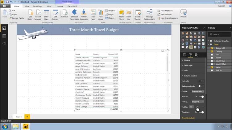
Next, let’s increase the font size to 12 point, using Format > Values > Text Size; and then Format > Column Headers > Text Size.
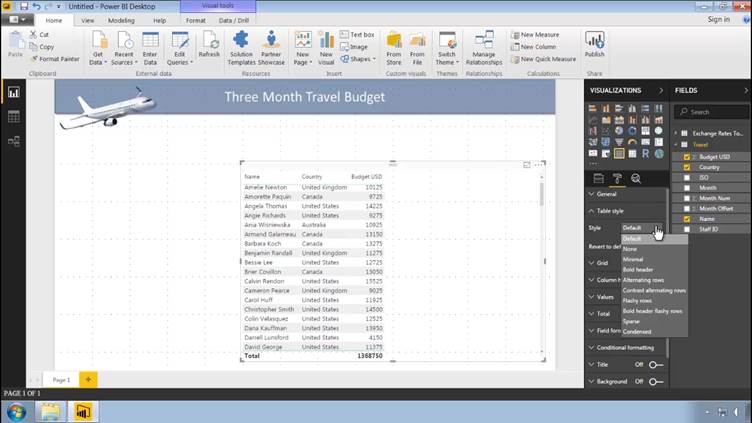
Finally, let’s spruce up the table formatting by choosing Format > Table Style > Condensed.
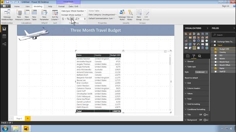
To format the numbers, to make them easier to read, simply click on the field in question (in this case, we highlight “Budget USD”) and, in the Modelling Tab, you will see a few icons which are very reminiscent of the formatting options you find in Excel. So, here, we can use the thousands separator option and set the number of decimals set to zero.
Creating Calculated Columns
Next, let’s use the data that we retrieved from the website to create columns which convert the budget figure into each of the other four currencies. We will do this by creating a series of DAX formulas. We will discuss DAX in more detail in later posts. For the moment, we will just create the formulas without too much discussion of DAX.
The best way to do create calculated columns is in Data mode. On the left of the screen, click on the Data button and then in the Fields pane, highlight the “Travel” table.
Now, although creating calculated columns may seem fairly similar to the operation which we performed in the Query Editor, there is one big difference: relationships. When creating a calculated column, we can use the relationship which Power BI automatically created to pull data across from the related table.
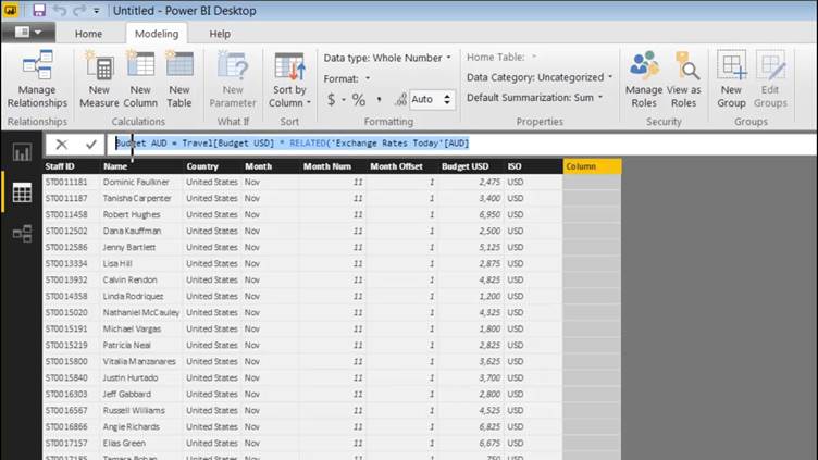
Let’s begin with the Australian dollars column; to calculate the travel budget figure in Australian dollars, we simply take budget USD column and multiply it by the AUD column in the related “Exchange Rates Today” table. The DAX formula that we need is as follows:
Budget AUD = Travel [Budget USD] * RELATED(‘Exchange Rates Today'[AUD])
First, we have the name of the function “Budget AUD” (This is our creation; we can use any name we choose.) Then, to refer to columns in a DAX formula, you use the name of the table (in single quotes if the name contains spaces) followed by the name the column in square brackets. However, because we are creating a column in the Travel table, when we refer to the AUD column of the “Exchange Rates Today” table, we need to wrap the column reference inside the RELATED function.
Power BI facilitates the creation of DAX formulas by displaying tooltips as you type. When the option that you need is displayed, you can simply highlight it, using the down arrow on your keyboard, then press the Tab key to insert it into your formula.
Since the formulas for calculating the budget figure in each of the other currencies will be very similar to the one which we have just created, it makes sense to copy it, using Control-C. (Right-click is not available in the formula bar.)
To create the Budget CAD column, simply click on New Column; press Control-V to paste in the first formula; then change “AUD” to “CAD” twice; once to rename the formula, and once to change the column being referenced. Your second formula should read:
Budget CAD = Travel [Budget USD] * RELATED(‘Exchange Rates Today'[CAD])
To finish, create two further columns, using the following formulas:
Budget GBP = Travel [Budget USD] * RELATED(‘Exchange Rates Today'[GBP])
And
Budget NZD = Travel [Budget USD] * RELATED(‘Exchange Rates Today'[NZD])
Using The Slicer Visual
Let us complete the report by adding a couple of slicers to enable the user to filter the data displayed in the table. To create a new visual, make sure that nothing is selected by clicking in space. The slicer visual is the icon which contains a funnel.
To populate the new visual, while it is still highlighted, in the Fields pane, click on the checkbox next to Country in the Travel table.
The text is fairly small by default. To increase the size use the slider in Format > Items > Text Size. The header is superfluous; so simply click the On/Off button next to its name to get rid of it.
To create a second slicer for Month, we can copy the one we have just customized. Right-click is not available; so just use Control-C, followed by Control-V. Then, to replace Country with Month, drag Travel > Month from the Fields pane on top of the Country field in the Fields Tab of the Visualizations pane.
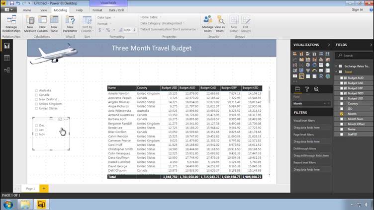
You will notice that the months are sorted alphabetically; to sort the months chronologically, we simply need a numeric column. If you switch to Data mode and highlight the Travel table, you will notice that we have a column called “Month Offset”. This indicates how many months in the future the budget figure in each row will apply.
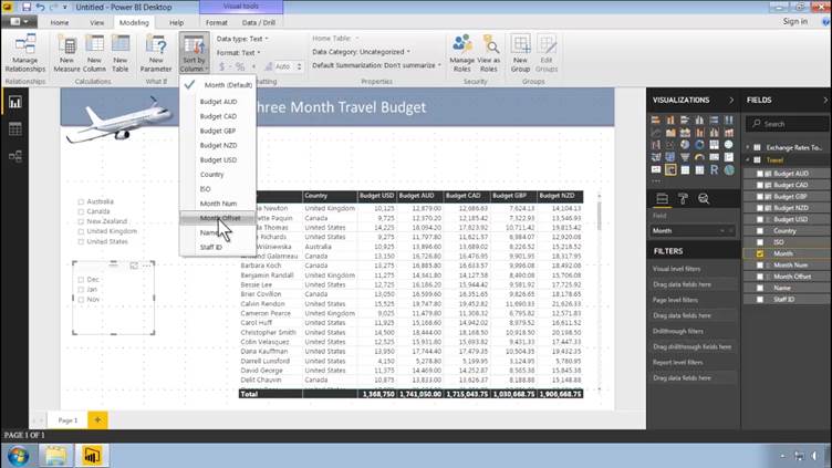
To have the months sorted using the numeric sort order of the “Month Offset” column, we highlight the “Month” column in the Fields pane; and, in the Modelling Tab of the Ribbon, Power BI has this very useful feature: Sort by Column. We simply choose “Month Offset” from the drop-down menu; and, thereafter, the “Month” column will be sorted using the values in the “Month Offset” column.
That completes our basic report.
So now, if we want to know how much Australia is going to be spending in November, for example; we can just use our two filters to restrict the data to those two criteria; and every time we refresh the report, we will be using the current currency conversion figures.